Motivation
Tree-based models like Random Forest and XGBoost have become very popular in solving tabular(structured) data problems and gained a lot of tractions in Kaggle competitions lately. It has its very deserving reasons. However, in this article, I want to introduce a different approach from fast.ai’s Tabular module leveraging:
Deep Learning and Embedding Layers.
This is a bit against industry consensus that Deep Learning is more for unstructured data like image, audio or NLP, and usually not suitable for handling tabular data. Yet, the introduction of embedding layers for the categorical data changed this perspective and we’ll try to use fast.ai’s tabular module on the Blue Book Bulldozers Competition on Kaggle and see how far this approach can go.
You can find the Kaggle Notebook 📔: here.
Loading Data

First, let’s import the necessary modules. The core one here is fastai.tabular:
from fastai import *
from fastai.tabular import *
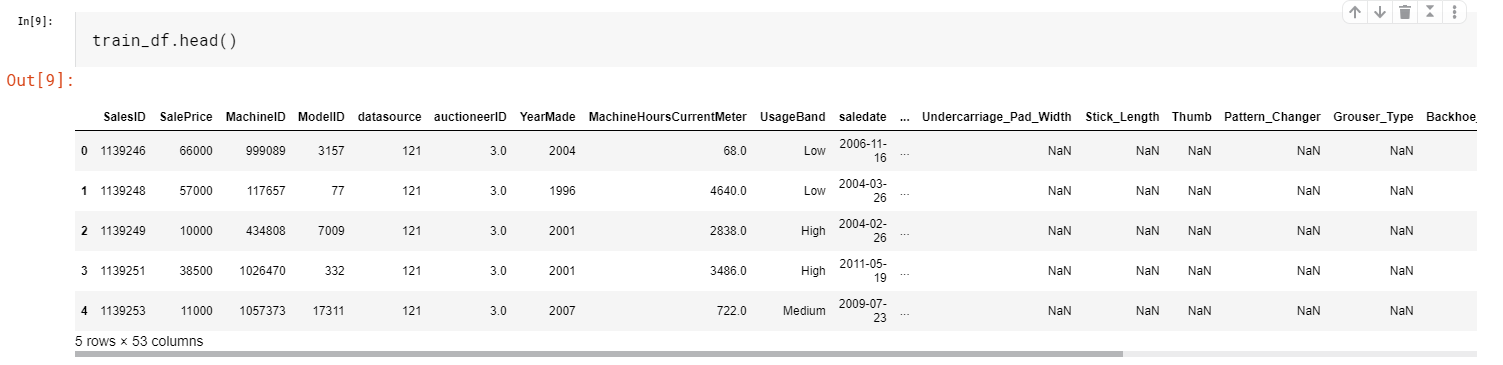
Then we’ll read the data into a Pandas DataFrame. You can find the specific code in the Kaggle Notebook link on top of this article but for here, I’ll only show necessary code snippets to keep things as concise as possible. We will read in the CSV file into train_df and this will be the DataFrame we’ll be mainly working on. We will also read in test_df which is the test set.
Let’s take a brief look at the data we’re dealing with:
len(train_df), len(test_df)
(401125, 12457)
Sorting the Training Set
This is to create a good validation set. It cannot be emphasized enough how important a good validation set is in making a successful model. Since we are predicting sales price data in the future, we need to make a validation set that all of its data is collected in the ‘future’ of the training set. So we need to sort the training set first, then split the ‘future’ part as the validation set.
Data Pre-Processing
The competition’s evaluation methods use RMSLE (root mean squared log error). So if we take the log of our prediction, we can just use the good old RMSE as our loss function. It’s just easier this way.
train_df.SalePrice = np.log(train_df.SalePrice)
For Feature Engineering, since we will be using deep learning to tackle the problem and it is very good at feature extraction, we’ll only do it on the saledate. This is the advantage of using a Deep Learning approach, it requires way less feature engineering and less dependent on domain knowledge. We’ll use the fast.ai’s add_datepart function to for adding some more features related to the sale date.
# The only feature engineering we do is add some meta-data from the sale date column, using 'add_datepart' function in fast.ai
add_datepart(train_df, "saledate", drop=False)
add_datepart(test_df, "saledate", drop=False)
What add_datepart does is it takes the saledate column and added a bunch of other columns like day of week, day of month, whether it is the start or end of a month, quarter and year, etc. These added features will offer more insights into the date and are relevant to user purchasing behaviors. For example, at the end of the year, the company will usually run promotions and prices will usually decrease.
Let’s check whether all these date related features got added into our DataFrame:
# check and see whether all date related meta data is added.
def display_all(df):
    with pd.option_context("display.max_rows", 1000, "display.max_columns", 1000):
        display(df)

display_all(train_df.tail(10).T)
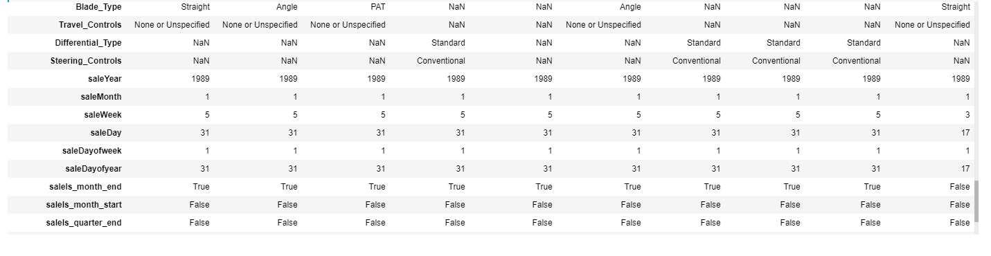
They did get added. Good. Now we need to do some data pre-processing since this DataFrame has quite some missing data and we also want to categorify and normalize the columns. With the fast.ai library, this is rather simple. We just specify the pre-processing methods we want into a Python list, like so:
# Defining pre-processing we want for our fast.ai DataBunch
procs=[FillMissing, Categorify, Normalize]
This variable procs will later be used to create the fast.ai DataBunch for training.
Building the Model
Let’s look at the data types of each column to decide which ones are categorical and which ones are continuous:
train_df.dtypes
g = train_df.columns.to_series().groupby(train_df.dtypes).groups
g
Here are the results:
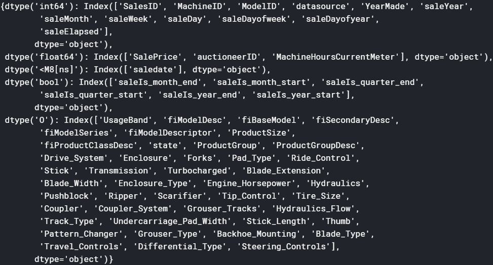
Then we’ll put all categorical columns into a list cat_vars and all continuous columns into a list cont_vars. These two variables will also be used to construct fast.ai DataBunch.
# prepare categorical and continous data columns for building Tabular DataBunch.
cat_vars = ['SalesID', 'YearMade', 'MachineID', 'ModelID', 'datasource', 'auctioneerID', 'UsageBand', 'fiModelDesc', 'fiBaseModel', 'fiSecondaryDesc', 'fiModelSeries', 'fiModelDescriptor', 'ProductSize',
            'fiProductClassDesc', 'state', 'ProductGroup', 'ProductGroupDesc', 'Drive_System', 'Enclosure', 'Forks', 'Pad_Type', 'Ride_Control', 'Stick', 'Transmission', 'Turbocharged', 'Blade_Extension',
            'Blade_Width', 'Enclosure_Type', 'Engine_Horsepower', 'Hydraulics', 'Pushblock', 'Ripper', 'Scarifier', 'Tip_Control', 'Tire_Size', 'Coupler', 'Coupler_System', 'Grouser_Tracks', 'Hydraulics_Flow',
            'Track_Type', 'Undercarriage_Pad_Width', 'Stick_Length', 'Thumb', 'Pattern_Changer', 'Grouser_Type', 'Backhoe_Mounting', 'Blade_Type', 'Travel_Controls', 'Differential_Type', 'Steering_Controls',
            'saleYear', 'saleMonth', 'saleWeek', 'saleDay', 'saleDayofweek', 'saleDayofyear', 'saleIs_month_end', 'saleIs_month_start', 'saleIs_quarter_end', 'saleIs_quarter_start', 'saleIs_year_end',
            'saleIs_year_start'
           ]

cont_vars = ['MachineHoursCurrentMeter', 'saleElapsed']
We’ll create another DataFrame df to feed into the DataBunch. We also specify the dependent variable as dep_var .
# rearrange training set before feed into the databunch
dep_var = 'SalePrice'
df = train_df[cat_vars + cont_vars + [dep_var,'saledate']].copy()
Now is the time to create our validation set. We do this by cutting out a block of the most recent entries from the training set. How big the block should be? Well, the same size as the test set. Let’s see the code:
# Look at the time period of test set, make sure it's more recent
test_df['saledate'].min(), test_df['saledate'].max()

# Calculate where we should cut the validation set. We pick the most recent 'n' records in training set where n is the number of entries in test set.
cut = train_df['saledate'][(train_df['saledate'] == train_df['saledate'][len(test_df)])].index.max()
cut

12621

# specify the valid_idx variable as the cut out range.
valid_idx = range(cut)
We first look at the time period of the test set and make sure it is more recent than all our training set. Then we calculate how many records we need to cut out.
Finally, let’s construct our DataBunch for training using fast.ai’s datablock API:
# Use fast.ai datablock api to put our training data into the DataBunch, getting ready for training
data = (TabularList.from_df(df, path=path, cat_names=cat_vars, cont_names=cont_vars, procs=procs)
                   .split_by_idx(valid_idx)
                   .label_from_df(cols=dep_var, label_cls=FloatList)
                   .databunch())
Building the Model
We will fire up a fast.ai tabular.learner from the DataBunch we just created. We want to limit the price range for our prediction to be within the history sale price range, so we need to calculate the y_range. Note that we multiplied the maximum of SalePrice by 1.2 so when we apply sigmoid, the upper limit will also be covered. This is a small trick to squeeze a bit more performance out of the model.
max_y = np.max(train_df['SalePrice'])*1.2
y_range = torch.tensor([0, max_y], device=defaults.device)
y_range

tensor([ 0.0000, 14.2363], device='cuda:0')
Now we can create our learner:
# Create our tabular learner. The dense layer is 1000 and 500 two layer NN. We used dropout, hai
learn = tabular_learner(data, layers=[1000,500], ps=[0.001,0.01], emb_drop=0.04, y_range=y_range, metrics=rmse)
The single most important thing about fast.ai tabular_learner is the use of embedding layers for categorical data. This is the ‘secret sauce’ that enables Deep Learning to be competitive in handling tabular data. With one embedding layer for each categorical variable, we introduced good interaction for the categorical variables and leverage Deep Learning’s biggest strength: Automatic Feature Extraction. We also used Drop Out for both the dense layers and embedding layers for better regularization. The metrics of the learner is RMSE since we’ve already taken the log of SalePrice. Let’s look at the model.
TabularModel(
  (embeds): ModuleList(
    (0): Embedding(388505, 600)
    (1): Embedding(72, 18)
    (2): Embedding(331868, 600)
    (3): Embedding(5155, 192)
   ...
    (60): Embedding(3, 3)
    (61): Embedding(2, 2)
    (62): Embedding(3, 3)
  )
  (emb_drop): Dropout(p=0.04, inplace=False)
  (bn_cont): BatchNorm1d(2, eps=1e-05, momentum=0.1, affine=True, track_running_stats=True)
  (layers): Sequential(
    (0): Linear(in_features=2102, out_features=1000, bias=True)
    (1): ReLU(inplace=True)
    (2): BatchNorm1d(1000, eps=1e-05, momentum=0.1, affine=True, track_running_stats=True)
    (3): Dropout(p=0.001, inplace=False)
    (4): Linear(in_features=1000, out_features=500, bias=True)
    (5): ReLU(inplace=True)
    (6): BatchNorm1d(500, eps=1e-05, momentum=0.1, affine=True, track_running_stats=True)
    (7): Dropout(p=0.01, inplace=False)
    (8): Linear(in_features=500, out_features=1, bias=True)
  )
)
As can be seen from the above, we have embedding layers for categorical columns, then followed by a drop out layer. We have a batch norm layer for the continuous columns, then we concatenate all of them (categorical embeddings + continuous variables) together and throw them into two fully connected layers with 1000 and 500 nodes, with Relu, BatchNorm, and Dropout in between. Quite standard stuff.
Now that we have the model, let’s use fast.ai’s learning rate finder to find a good learning rate:
learn.lr_find()
learn.recorder.plot()
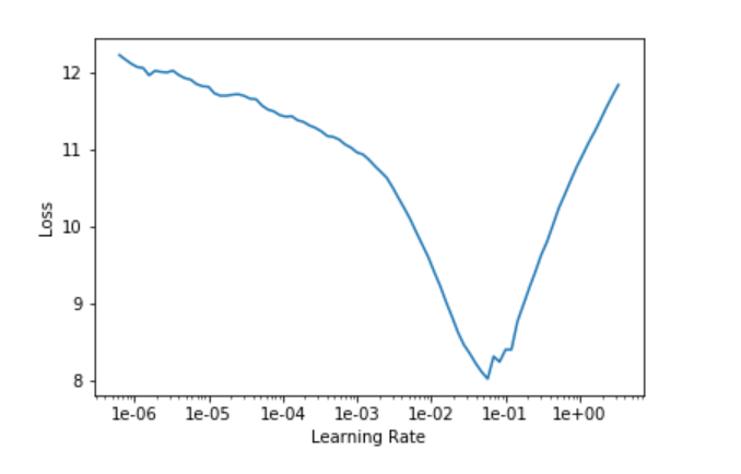
We’ll pick the learning rate at the end of the biggest learning rate curve slope: le-02
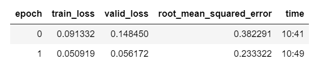
Let’s do some training using fast.ai’s One-Cycle Training approach. Note that we added some weight decay (0.2) for regularization.
learn.fit_one_cycle(2, 1e-2, wd=0.2)
We can train some more cycles with smaller learning rate:
learn.fit_one_cycle(5, 3e-4, wd=0.2)
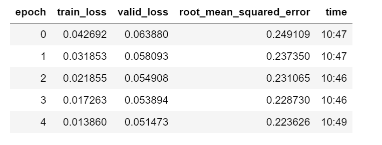
We’ve reached a score of 0.223 on our validation set. Since the competition is not accepting submissions, we can only look at the leaderboard to get a rough idea of how well this model performs:
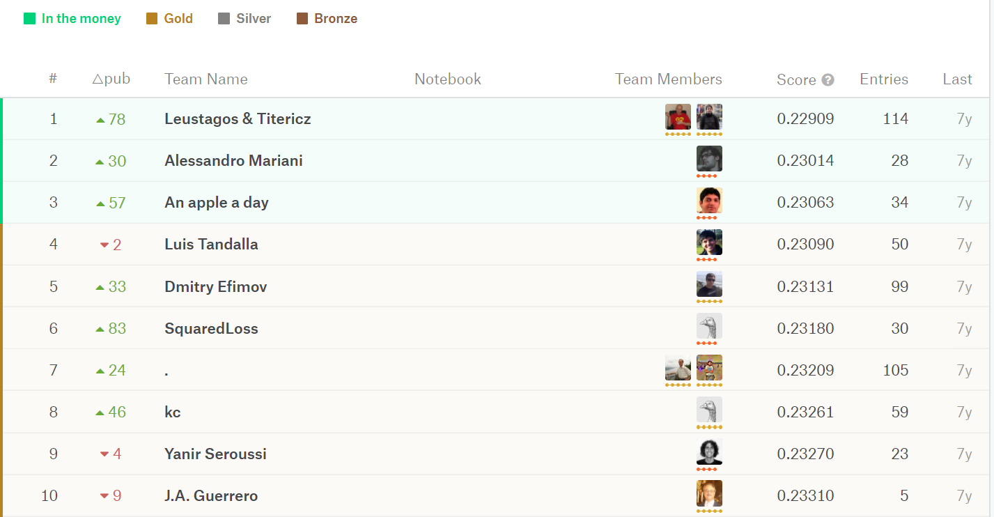
The top place is 0.229. Compare to this model’s 0.223. We don’t know how well it works on the test set but overall I think the result we got isn’t bad at all.
A Couple of More Words on Embedding Layers
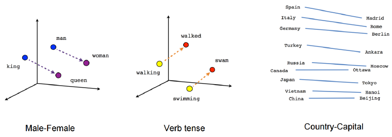
What makes everything click here is the embedding layers. Embedding is just a fancy word of saying mapping something to a vector. Like the word embedding that is getting more popular in NLP, it means using a vector (the size is arbitrary though, depending on tasks) to represent words, and those vectors are weights and can be trained via back-prop.
Similarly, for our case, we used embeddings on our categorical variables. Each column gets an embedding matrix that can be trained. And each unique column value gets a specific vector mapped to it. The beautiful thing about this is: with embedding, we can now develop ‘semantics’ to the variable, ‘semantics’ in the form of weights that matters to our sale price and can be extracted and trained via our deep neural network. The model will have the ‘depth’ it needs to fit a big data set well.
But don’t take my words for it, or just look at the results of my humble little project. In a more glory case, there was this paper by the folks who came 3rd in a Kaggle competition for something called Rossman (prediction future sales). Among the top teams in the leaderboard, everyone else used some kind of heavy feature engineering, but by using embedding layers, they managed to score 3rd place with way less feature engineering.
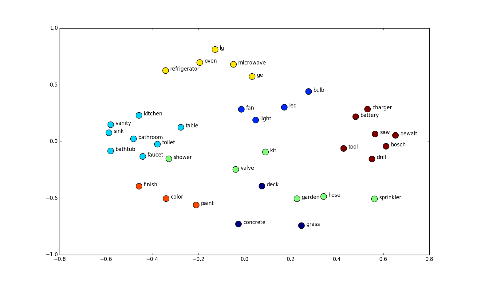
What’s more interesting is, with embedding layers, you can actually visualize the variable projection in the embedding matrix space. Take the Rossman project as an example. They took a two-dimensional projection of the embedding matrix for the German states.
And if you circle some states on the embedding space and same states on the actual map. You’ll find out that they are scarily similar. The embedding layer actually discovered geography.