
When it comes to frameworks in technology, one interesting thing is that from the very beginning, there always seems to be a variety of choices. But over time, the competitions will evolve into having only two strong contenders left. Cases in point being ‘PC vs Mac’, ‘iOS vs Android’, ‘React.js vs Vue.js’, etc. And now, we have ‘PyTorch vs TensorFlow’ in machine learning.
TensorFlow, backed by Google, is undoubtedly the front-runner here. Released in 2015 as an open-source machine learning framework, it quickly gained a lot of attention and acceptance, especially in industries where production readiness and deployment is key. PyTorch is introduced much later by Facebook in 2017 but quickly gaining a lot of love from practitioners and researchers because of its dynamic computational graph and ‘pythonic’ style.
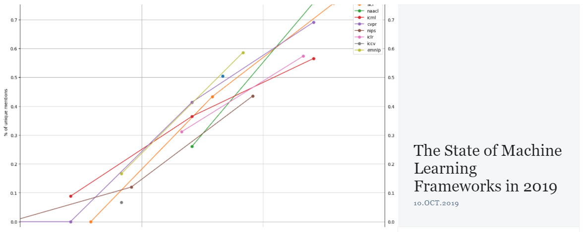
Image from The Gradient
Recent research by The Gradient shows that PyTorch is doing great with researchers and TensorFlow is dominating the industry world:
In 2019, the war for ML frameworks has two remaining main contenders: PyTorch and TensorFlow. My analysis suggests that researchers are abandoning TensorFlow and flocking to PyTorch in droves. Meanwhile in industry, Tensorflow is currently the platform of choice, but that may not be true for long. — The Gradient
The recent release of PyTorch 1.3 introduced PyTorch Mobile, quantization and other goodies that are all in the right direction to close the gap. If you are somewhat familiar with neural network basics but want to try PyTorch as a different style, then please read on. I’ll try to explain how to build a Convolutional Neural Network classifier from scratch for the Fashion-MNIST dataset using PyTorch. The code here can be used on Google Colab and Tensor Board if you don’t have a powerful local environment. Without further ado, let’s get started. You can find the Google Colab Notebook and GitHub link below:
👽 GitHub
Import
First, let’s import the necessary modules.
    # import standard PyTorch modules
    import torch
    import torch.nn as nn
    import torch.nn.functional as F
    import torch.optim as optim
    from torch.utils.tensorboard import SummaryWriter # TensorBoard support

    # import torchvision module to handle image manipulation
    import torchvision
    import torchvision.transforms as transforms

    # calculate train time, writing train data to files etc.
    import time
    import pandas as pd
    import json
    from IPython.display import clear_output

    torch.set_printoptions(linewidth=120)
    torch.set_grad_enabled(True)     # On by default, leave it here for clarity
PyTorch modules are quite straight forward.
torch
torch is the main module that holds all the things you need for **Tensor **computation. You can build a fully functional neural network using Tensor computation alone, but this is not what this article is about. We’ll make use of the more powerful and convenient torch.nn, torch.optim and torchvision classes to quickly build our CNN. For those of you interested in knowing how to do this from ‘scratch scratch’, visit this fantastic PyTorch official tutorial by Jeremy Howard.
torch.nn and torch.nn.functional

Photo by Alphacolor on Unsplash
The torch.nnmodule provides many classes and functions to build neural networks. You can think of it as the fundamental building blocks of neural networks: models, all kinds of layers, activation functions, parameter classes, etc. It allows us to build the model like putting some LEGO set together.
torch.optim
torch.optim offers all the optimizers like SGD, ADAM, etc., so you don’t have to write it from scratch.
torchvision
torchvision contains a lot of popular datasets, model architectures, and common image transformations for computer vision. We get our Fashion MNIST dataset from it and also use its transforms.
SummaryWriter (Tensor Board)
SummaryWriter enables PyTorch to generate the report for Tensor Board. We’ll use Tensor Board to look at our training data, compare results and gain intuition. Tensor Board used to be TensorFlow’s biggest advantage over PyTorch, but it is now officially supported by PyTorch from v1.2.
We also imported some other utility modules like time, json, pandas, etc.
Dataset
torchvision already has the Fashion MNIST dataset. If you’re not familiar with Fashion MNIST dataset:
Fashion-MNIST is a dataset of Zalando’s article images—consisting of a training set of 60,000 examples and a test set of 10,000 examples. Each example is a 28x28 grayscale image, associated with a label from 10 classes. We intend Fashion-MNIST to serve as a direct drop-in replacement for the original MNIST dataset for benchmarking machine learning algorithms. It shares the same image size and structure of training and testing splits. — From Github
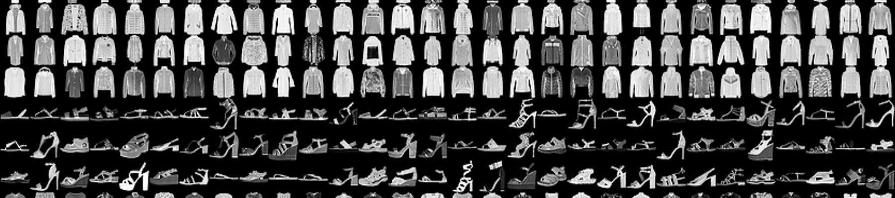
Fashion MNIST Dataset — From GitHub
    # Use standard FashionMNIST dataset
    train_set = torchvision.datasets.FashionMNIST(
        root = './data/FashionMNIST',
        train = True,
        download = True,
        transform = transforms.Compose([
            transforms.ToTensor()
        ])
    )
This doesn’t need much explanation. We specified the root directory to store the dataset, snatch the training data, allow it to be downloaded if not present at the local machine, and then apply the transforms.ToTensor to turn images into **Tensor **so we can directly use it with our network. The dataset is stored in the dataset class named train_set.
Network
Building the actual neural network in PyTorch is fun and easy. I assume you have some basic concept of how a Convolutional Neural Network works. If you don’t, you can refer to this video from deeplizard:
The Fashion MNIST is only 28x28 px in size, so we actually don’t need a very complicated network. We can just build a simple CNN like this:
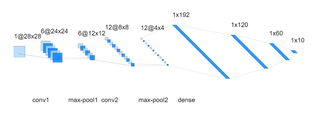
We have two convolution layers, each with 5x5 kernels. After each convolution layer, we have a max-pooling layer with a stride of 2. This allows us to extract the necessary features from the images. Then we flatten the tensors and put them into a dense layer, pass through a Multi-Layer Perceptron (MLP) to carry out the task of classification of our 10 categories.
Now that we are clear about the structure of the network, let’s see how we can use PyTorch to build it:
    # Build the neural network, expand on top of nn.Module
    class Network(nn.Module):
      def __init__(self):
        super().__init__()

        # define layers
        self.conv1 = nn.Conv2d(in_channels=1, out_channels=6, kernel_size=5)
        self.conv2 = nn.Conv2d(in_channels=6, out_channels=12, kernel_size=5)

        self.fc1 = nn.Linear(in_features=12*4*4, out_features=120)
        self.fc2 = nn.Linear(in_features=120, out_features=60)
        self.out = nn.Linear(in_features=60, out_features=10)

      # define forward function
      def forward(self, t):
        # conv 1
        t = self.conv1(t)
        t = F.relu(t)
        t = F.max_pool2d(t, kernel_size=2, stride=2)

        # conv 2
        t = self.conv2(t)
        t = F.relu(t)
        t = F.max_pool2d(t, kernel_size=2, stride=2)

        # fc1
        t = t.reshape(-1, 12*4*4)
        t = self.fc1(t)
        t = F.relu(t)

        # fc2
        t = self.fc2(t)
        t = F.relu(t)

        # output
        t = self.out(t)
        # don't need softmax here since we'll use cross-entropy as activation.

        return t
First of all, all network classes in PyTorch expand on the base class: nn.Module. It packs all the basics: weights, biases, forward method and also some utility attributes and methods like .parameters() and .zero_grad()which we will be using too.
The structure of our network is defined in the init dunder function.
    def __init__(self):
      super().__init__()

      # define layers
      self.conv1 = nn.Conv2d(in_channels=1, out_channels=6, kernel_size=5)
      self.conv2 = nn.Conv2d(in_channels=6, out_channels=12, kernel_size=5)
      self.fc1 = nn.Linear(in_features=12*4*4, out_features=120)
      self.fc2 = nn.Linear(in_features=120, out_features=60)
      self.out = nn.Linear(in_features=60, out_features=10)
nn.Conv2d and nn.Linear are two standard PyTorch layers defined within the torch.nn module. These are quite self-explanatory. One thing to note is that we only defined the actual layers here. The activation and max-pooling operations are included in the forward function that is explained below.
    # define forward function
    def forward(self, t):
      # conv 1
      t = self.conv1(t)
      t = F.relu(t)
      t = F.max_pool2d(t, kernel_size=2, stride=2)

      # conv 2
      t = self.conv2(t)
      t = F.relu(t)
      t = F.max_pool2d(t, kernel_size=2, stride=2)

      # fc1
      t = t.reshape(-1, 12*4*4)
      t = self.fc1(t)
      t = F.relu(t)

      # fc2
      t = self.fc2(t)
      t = F.relu(t)

      # output
      t = self.out(t)

      # don't need softmax here since we'll use cross-entropy as activation.
      return t
Once the layer is defined, we can then use the layer itself to compute the forward results of each layer, coupled with the activation function(ReLu) and Max Pooling operations, we can easily write the forward function of our network as above. Notice that on fc1(Fully Connect layer 1), we used PyTorch’s tensor operation t.reshape to flatten the tensor so it can be passed to the dense layer afterward. Also, we didn’t add the softmax activation function at the output layer since PyTorch’s CrossEntropy function will take care of that for us.
Hyperparameters
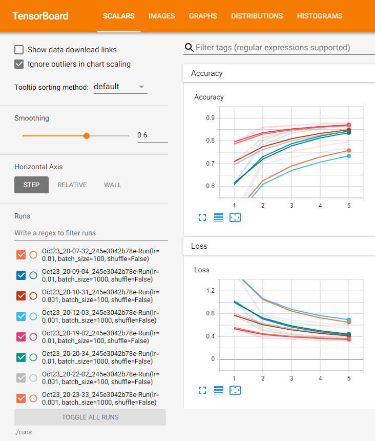
Normally, we can just handpick one set of hyperparameters and do some experiments with them. In this example, we want to do a bit more by introducing some structuring. We’ll build a system to generate different hyperparameter combinations and use them to carry out training ‘runs’. Each ‘run’ uses one set of hyperparameter combinations. Export the training data/results of each run to Tensor Board so we can directly compare and see which hyperparameters set performs the best.
We store all our hyperparameters in an **OrderedDict**:
    # put all hyper params into a OrderedDict, easily expandable
    params = OrderedDict(
        lr = [.01, .001],
        batch_size = [100, 1000],
        shuffle = [True, False]
    )
    epochs = 3
lr: Learning Rate. We want to try 0.01 and 0.001 for our models.
batch_size: Batch Size to speed up the training process. We’ll use 100 and 1000.
shuffle: Shuffle toggle, whether we shuffle the batch before training.
Once the parameters are down. We use two helper classes: RunBuilder and RunManager to manage our hyperparameters and training process.
RunBuilder
The main purpose of the class RunBuilder is to offer a static method get_runs. It takes the OrderedDict (with all hyperparameters stored in it) as a parameter and generates a named tuple Run, each element of runrepresent one possible combination of the hyperparameters. This named tuple is later consumed by the training loop. The code is easy to understand.
    # import modules to build RunBuilder and RunManager helper classes
    from collections  import OrderedDict
    from collections import namedtuple
    from itertools import product

    # Read in the hyper-parameters and return a Run namedtuple containing all the
    # combinations of hyper-parameters
    class RunBuilder():
      @staticmethod
      def get_runs(params):

        Run = namedtuple('Run', params.keys())

        runs = []
        for v in product(*params.values()):
          runs.append(Run(*v))

        return runs
RunManager
There are four main purposes of the RunManager class.
-
Calculate and record the duration of each epoch and run.
-
Calculate the training loss and accuracy of each epoch and run.
-
Record the training data (e.g. loss, accuracy, weights, gradients, computational graph, etc.) for each epoch and run, then export them into Tensor Board for further analysis.
-
Save all training results in csv and json for future reference or API extraction.
As you can see, it helps us take care of the logistics which is also important for our success in training the model. Let’s look at the code. It’s a bit long so bear with me:
# Helper class, help track loss, accuracy, epoch time, run time,
# hyper-parameters etc. Also record to TensorBoard and write into csv, json
class RunManager():
def __init__(self):
# tracking every epoch count, loss, accuracy, time
self.epoch_count = 0
self.epoch_loss = 0
self.epoch_num_correct = 0
self.epoch_start_time = None
# tracking every run count, run data, hyper-params used, time
self.run_params = None
self.run_count = 0
self.run_data = []
self.run_start_time = None
# record model, loader and TensorBoard
self.network = None
self.loader = None
self.tb = None
# record the count, hyper-param, model, loader of each run
# record sample images and network graph to TensorBoard
def begin_run(self, run, network, loader):
self.run_start_time = time.time()
self.run_params = run
self.run_count += 1
self.network = network
self.loader = loader
self.tb = SummaryWriter(comment=f'-{run}')
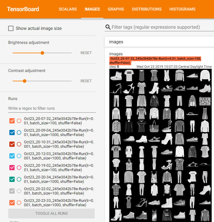
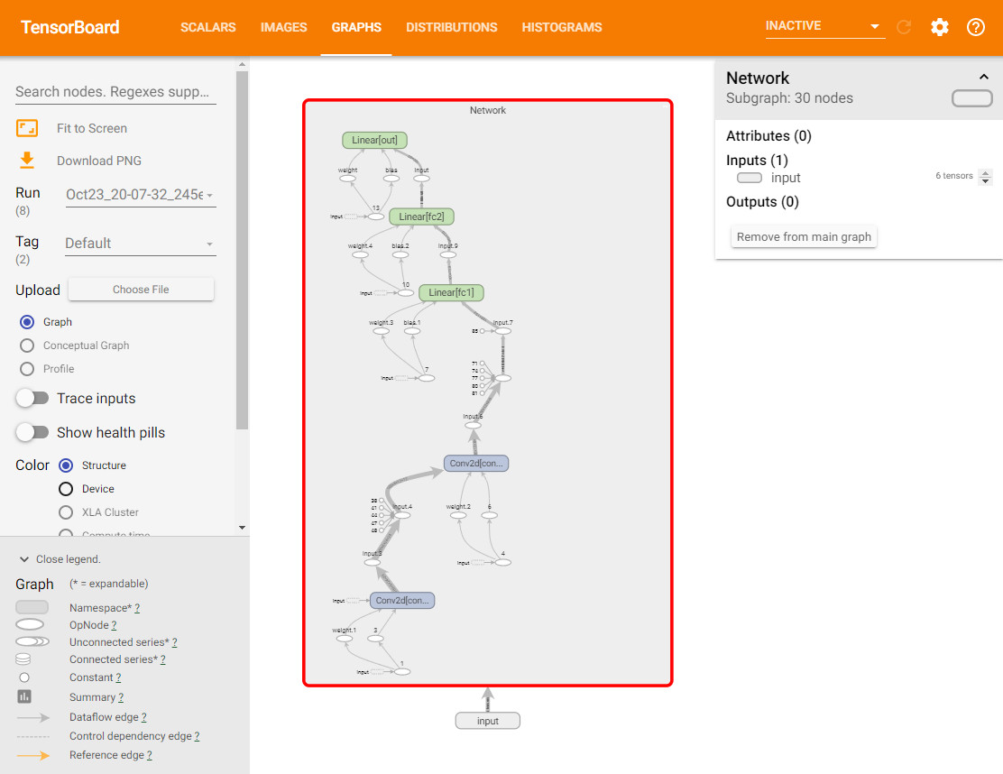
images, labels = next(iter(self.loader))
grid = torchvision.utils.make_grid(images)
self.tb.add_image('images', grid)
self.tb.add_graph(self.network, images)
# when run ends, close TensorBoard, zero epoch count
def end_run(self):
self.tb.close()
self.epoch_count = 0
# zero epoch count, loss, accuracy,
def begin_epoch(self):
self.epoch_start_time = time.time()
self.epoch_count += 1
self.epoch_loss = 0
self.epoch_num_correct = 0
#
def end_epoch(self):
# calculate epoch duration and run duration(accumulate)
epoch_duration = time.time() - self.epoch_start_time
run_duration = time.time() - self.run_start_time
# record epoch loss and accuracy
loss = self.epoch_loss / len(self.loader.dataset)
accuracy = self.epoch_num_correct / len(self.loader.dataset)
# Record epoch loss and accuracy to TensorBoard
self.tb.add_scalar('Loss', loss, self.epoch_count)
self.tb.add_scalar('Accuracy', accuracy, self.epoch_count)
# Record params to TensorBoard
for name, param in self.network.named_parameters():
self.tb.add_histogram(name, param, self.epoch_count)
self.tb.add_histogram(f'{name}.grad', param.grad, self.epoch_count)
# Write into 'results' (OrderedDict) for all run related data
results = OrderedDict()
results["run"] = self.run_count
results["epoch"] = self.epoch_count
results["loss"] = loss
results["accuracy"] = accuracy
results["epoch duration"] = epoch_duration
results["run duration"] = run_duration
# Record hyper-params into 'results'
for k,v in self.run_params._asdict().items(): results[k] = v
self.run_data.append(results)
df = pd.DataFrame.from_dict(self.run_data, orient = 'columns')
# display epoch information and show progress
clear_output(wait=True)
display(df)
# accumulate loss of batch into entire epoch loss
def track_loss(self, loss):
# multiply batch size so variety of batch sizes can be compared
self.epoch_loss += loss.item() * self.loader.batch_size
# accumulate number of corrects of batch into entire epoch num_correct
def track_num_correct(self, preds, labels):
self.epoch_num_correct += self._get_num_correct(preds, labels)
@torch.no_grad()
def _get_num_correct(self, preds, labels):
return preds.argmax(dim=1).eq(labels).sum().item()
# save end results of all runs into csv, json for further analysis
def save(self, fileName):
pd.DataFrame.from_dict(
self.run_data,
orient = 'columns',
).to_csv(f'{fileName}.csv')
with open(f'{fileName}.json', 'w', encoding='utf-8') as f:
json.dump(self.run_data, f, ensure_ascii=False, indent=4)
init: Initialize necessary attributes like count, loss, number of correct predictions, start time, etc.
begin_run: Record run start time so when a run is finished, the duration of the run can be calculated. Create a SummaryWriter object to store everything we want to export into Tensor Board during the run. Write the network graph and sample images into the SummaryWriter object.
end_run: When run is finished, close the SummaryWriter object and reset the epoch count to 0 (getting ready for next run).
begin_epoch: Record epoch start time so epoch duration can be calculated when epoch ends. Reset epoch_loss and epoch_num_correct.
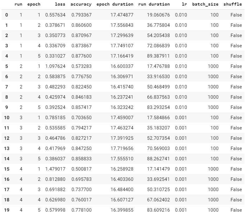
end_epoch: This function is where most things happen. When an epoch ends, we’ll calculate the epoch duration and the run duration(up to this epoch, not the final run duration unless for the last epoch of the run). We’ll calculate the total loss and accuracy for this epoch, then export the loss, accuracy, weights/biases, gradients we recorded into Tensor Board. For ease of tracking within the Jupyter Notebook, we also created an OrderedDict object results and put all our run data(loss, accuracy, run count, epoch count, run duration, epoch duration, all hyperparameters) into it. Then we’ll use **Pandas **to read it in and display it in a neat table format.
track_loss, track_num_correct, _get_num_correct: These are utility functions to accumulate the loss, number of correct predictions of each batch so the epoch loss and accuracy can be calculated later.
save: Save all run data (a list of results **OrderedDict **objects for all runs) into csv and json format for further analysis or API access.
There is a lot to take in for this RunManager class. Congrats on coming to this far! The hardest part is already behind you. From now on everything will start to come together and make sense.
Training
Finally, we are ready to do some training! With the help of our RunBuilder and RunManager classes, the training process is a breeze:
    m = RunManager()

    # get all runs from params using RunBuilder class
    for run in RunBuilder.get_runs(params):

        # if params changes, following line of code should reflect the changes too
        network = Network()
        loader = torch.utils.data.DataLoader(train_set, batch_size = run.batch_size)
        optimizer = optim.Adam(network.parameters(), lr=run.lr)

        m.begin_run(run, network, loader)
        for epoch in range(epochs):

          m.begin_epoch()
          for batch in loader:

            images = batch[0]
            labels = batch[1]
            preds = network(images)
            loss = F.cross_entropy(preds, labels)

            optimizer.zero_grad()
            loss.backward()
            optimizer.step()

            m.track_loss(loss)
            m.track_num_correct(preds, labels)

          m.end_epoch()
        m.end_run()

    # when all runs are done, save results to files
    m.save('results')
First, we use RunBuilder to create an iterator of hyperparameters, then loop through each hyperparameter combination to carry out our training:
for run in RunBuilder.get_runs(params):
Then, we create our network object from the Network class defined above. network = Network() . This network objects hold all our weights/biases we need to train.
We also need to create a DataLoader object. It is a PyTorch class that holds our training/validation/test dataset, and it will iterate through the dataset and gives us training data in batches equal to the batch_size specied.
loader = torch.utils.data.DataLoader(train_set, batch_size = run.batch_size)
After that, we’ll create an optimizer using torch.optim class. The optim class gets network parameters and learning rate as input and will help us step through the training process and updates the gradients, etc. We’ll use Adam as our optimization algorithm here.
optimizer = optim.Adam(network.parameters(), lr=run.lr)
OK. Now we have our network created, data loader prepared and optimizer chosen. Let’s get the training rolling!
We will loop through all the epochs we want (3 here) to train, so we wrap everything in an ‘epoch’ loop. We also use the begin_run method of our RunManager class to start tracking run training data.
    m.begin_run(run, network, loader)
    for epoch in range(epochs):
For each epoch, we’ll loop through each batch of images to carry out the training.
    m.begin_epoch()
    for batch in loader:
      images = batch[0]
      labels = batch[1]
      preds = network(images)
      loss = F.cross_entropy(preds, labels)

      optimizer.zero_grad()
      loss.backward()
      optimizer.step()

      m.track_loss(loss)
      m.track_num_correct(preds, labels)
The above code is where real training happens. We read in the images and labels from the batch, use network class to do the forward propagation (remember the forward method above?) and get the predictions. With predictions, we can calculate the loss of this batch using cross_entropy function. Once the loss is calculated, we reset the gradients (otherwise PyTorch will accumulate the gradients which is not what we want) with .zero_grad(), do one back propagation use loss.backward()method to calculate all the gradients of the weights/biases. Then, we use the optimizer defined above to update the weights/biases. Now that the network is updated for the current batch, we’ll calculate the loss and number of correct predictions and accumulate/track them using track_loss and track_num_correct methods of our RunManager class.
Once all is finished, we’ll save the results in files usingm.save(‘results’).
The output of the runs in the notebook looks like this:
Tensor Board
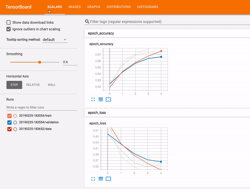
Image from Tensorboard.org
Tensor Board is a TensorFlow visualization tool now also supported by PyTorch. We’ve already taken the efforts to export everything into the ‘./runs’ folder where Tensor Board will be looking into for records to consume. What we need to do now is just to launch the Tensor Board and check. Since I’m running this model on Google Colab, we’ll use a service called ngrok to proxy and access our Tensor Board running on Colab virtual machine. Install ngrok first:
    !wget https://bin.equinox.io/c/4VmDzA7iaHb/ngrok-stable-linux-amd64.zip

    !unzip ngrok-stable-linux-amd64.zip
Then, specify the folder we want to run Tensor Board from and launch the Tensor Board web interface (./runs is the default):
    LOG_DIR = './runs'

    get_ipython().system_raw(

    'tensorboard --logdir {} --host 0.0.0.0 --port 6006 &'

    .format(LOG_DIR)

    )
Launch ngrok proxy:
get_ipython().system_raw('./ngrok http 6006 &')
Generate an URL so we can access our Tensor Board from within the Jupyter Notebook:
    ! curl -s http://localhost:4040/api/tunnels | python3 -c \

    "import sys, json; print(json.load(sys.stdin)['tunnels'][0]['public_url'])"
As we can see below, TensorBoard is a very convenient visualization tool for us to get insights into our training and can help greatly with the hyperparameter tuning process. We can easily spot which hyperparameter comp performs the best and then using it to do our real training.
Conclusion
As you can see, PyTorch as a machine learning framework is flexible, powerful and expressive. You just write Python code. Since the main focus of this article is to showcase how to use PyTorch to build a Convolutional Neural Network and training it in a structured way, I didn’t finish the whole training epochs and the accuracy is not optimum. You can try it yourself and see how well the model performs.
This article is heavily inspired by deeplizard’s PyTorch video series on YouTube. Even most of the code snippets are directly copied from it. I’d like to thank them for the great content and if you feel the need to delve down deeper, feel free to go check it out and subscribe to their channel.